Test Description
This test assesses how easy it is to access and run a UFS SRW Application configuration, modify the configuration to run a getting started step and two experiments:
- Different horizontal resolution, and
- New physics suite definition file (SDF).
You will be rerunning the code each time, and then comparing the results.
The test case used here is a two-consecutive day period with significant severe weather across the Contiguous United States (CONUS) from 15-16 June 2019. After completing the technical exercise, participants submit feedback on their experience through a short questionnaire. You don’t have to be a graduate student to take the test – all feedback is appreciated!
If you decide to take the test and have not yet registered, please register and submit your feedback here.
In order to perform the test, you will start by running the default SRW Application configuration using the GFSv15p2 suite definition file (SDF) for 48 hours starting at 00 UTC on 15 June 2019 on a 25-km predefined CONUS domain to establish a control experiment. Once that is successful, two additional experiments will be conducted.
First, you will change the configuration to run a 12-hour forecast starting at 18 UTC on 15 June 2019 on a 3-km predefined CONUS domain, still using the GFSv15p2 SDF. Next, you will run the same 12-hour forecast on the 2-km predefined domain, but this time you will use the RRFSv1alpha SDF. Working your way through these examples will assist you with learning how to change these settings and conduct new experiments. Python scripts are available to plot a variety of files from each run as well as difference those fields between two runs.
Important Note: If you are using a laptop for running the SRW App you will need a minimum of 4 Gb of memory and at least 40 Gb of disk space to run a 25 km resolution CONUS case. Running a 48 hour simulation will likely take several hours and thus you may wish to run 12 hour simulations instead. In addition, if you would like to run a 3 km resolution CONUS case you will need at least 24 Gb of memory and additional disk space depending on your forecast output frequency.
All information needed for running the SRW App GST is found in this document or through links provided below. In case you are interested in additional information, detailed documentation is provided in the SRW App User’s Guide.
Step 1 – Run the Control Case
Follow the instructions on the Getting Started page to clone the SRW App umbrella repository, build the application, generate the experiment, and run the workflow for the default case.
Case summary: 20190615, 00 UTC initialization, 48-hr forecast, 25-km CONUS domain, FV3_GFS_v15p2 suite definition file (SDF)
Example forecast plots are available here.
Step 2 – Run the horizontal resolution change experiment
The next experiment will have you run a case using the 3-km CONUS domain for a 12 hour forecast initialized at 18 UTC. In this case you will still use the same SDF (FV3_GFS_v15p2).
Experiment #1 summary: 20190615, 18 UTC initialization, 12-hr forecast, 3-km CONUS domain, FV3_GFS_v15p2 SDF
To start, you will need to generate a new workflow to run the next experiment. You can use the config.sh that was used for the control case as a starting point for this new experiment.
cd ufs-srweather-app/regional_workflow/ush
If you would like to save the original config.sh from your control case you can rename it.
cp config.sh config_gst_CONUS_25km_GFSv15p2.sh
Modify config.sh to update the settings to the following values:
	EXPT_SUBDIR="test_CONUS_3km_GFSv15p2" [new experiment output directory name]

PREDEF_GRID_NAME="RRFS_CONUS_3km" [move to the 3-km CONUS domain]

FCST_LEN_HRS="12" [shorten the forecast length to 12 hours]

LBC_SPEC_INTVL_HRS="3" [provide lateral boundary condition (LBC) files every 3 hours]

CYCL_HRS=( "18" ) [initialize case at 18 UTC]

WTIME_RUN_FCST="01:30:00" [increase the wall clock time]

EXTRN_MDL_FILES_LBCS=( "gfs.pgrb2.0p25.f003" "gfs.pgrb2.0p25.f006" "gfs.pgrb2.0p25.f009" "gfs.pgrb2.0p25.f012" ) [point to the 3-hourly LBC files]
Ensure you have loaded the appropriate python environment for the workflow as described in the Getting Started page:
source ufs-srweather-app/env/wflow_.env
And generate the new workflow:
./generate_FV3LAM_wflow.sh
Upon successful generation of the new workflow, go to the experiment directory (expt_dirs/test_CONUS_3km_GFSv15p2) and run the workflow as you did for the control case.
cd $EXPTDIR

./launch_FV3LAM_wflow.sh (-or- rocotorun -w FV3LAM_wflow.xml -d FV3LAM_wflow.db -v 10)
You can also use the Python plotting scripts to visualize the results for this experiment as you did for the control case.
Generate the python plots:
cd ufs-srweather-app/regional_workflow/ush/Python
Load the appropriate environment for your platform, as necessary, following the prior instructions.
To run the Python plotting script for a single run, six command line arguments are required. If the batch script is being used, multiple environment variables need to be set prior to submitting the script:
export HOMErrfs=/path-to/ufs-srweather-app/regional_workflow

export EXPTDIR=/path-to/expt_dirs/test_CONUS_3km_GFSv15p2
Note, while the setting for the HOMErrfs environment variable should not need to be changed from the previous case, the EXPTDIR will need to be updated to point to the new experiment directory (test_CONUS_3km_GFSv15p2). In addition, you might wish to change the following settings in the batch script for more frequent plots:
export FCST_START=3

export FCST_INC=3
Example plots are provided here.
Step 3 – Run the physics suite change experiment
The final experiment will again have you run a case using the 3-km CONUS domain for a 12 hour forecast initialized at 18 UTC. In this case you will use a new SDF called FV3_RRFS_v1alpha. See table below for details.
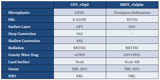
Experiment #2 summary: 20190615, 18 UTC initialization, 12-hr forecast, 3-km CONUS domain, FV3_RRFS_v1alpha SDF
Again, you will need to generate a new workflow to run the next experiment. You can use the config.sh that was used for the previous horizontal resolution change experiment case as a starting point for this new experiment.
If you would like to save the previous config.sh from your horizontal resolution change experiment you can rename it.
cp config.sh config_gst_CONUS_3km_GFSv15p2.sh
Modify config.sh to update the settings to the following values:
EXPT_SUBDIR="test_CONUS_3km_RRFSv1alpha"

PREDEF_GRID_NAME="RRFS_CONUS_3km" [should already be set based on previous experiment]

CCPP_PHYS_SUITE="FV3_RRFS_v1alpha"

LBC_SPEC_INTVL_HRS="1" [based on the IC/LBC data used for this experiment, this setting may be increased to a frequency of 1 hour, but it is not required.]

EXTRN_MDL_NAME_ICS="HRRR"

EXTRN_MDL_NAME_LBCS="RAP"

EXTRN_MDL_SOURCE_BASEDIR_ICS="/path-to/model_data/HRRR"

EXTRN_MDL_FILES_ICS=( "hrrr.wrfprsf00.grib2" )

EXTRN_MDL_SOURCE_BASEDIR_LBCS="/path-to/model_data/RAP"

EXTRN_MDL_FILES_LBCS=( "rap.wrfprsf01.grib2" "rap.wrfprsf02.grib2" "rap.wrfprsf03.grib2" "rap.wrfprsf04.grib2" "rap.wrfprsf05.grib2" "rap.wrfprsf06.grib2" "rap.wrfprsf07.grib2" "rap.wrfprsf08.grib2"  "rap.wrfprsf09.grib2" "rap.wrfprsf10.grib2" "rap.wrfprsf11.grib2" "rap.wrfprsf12.grib2")
Since we will be using HRRR/RAP IC/LBCs, the following two lines should be removed from the config.sh:
FV3GFS_FILE_FMT_ICS="grib2"

FV3GFS_FILE_FMT_LBCS="grib2"
Ensuring that the following settings remain the same as the horizontal resolution change experiment will enable a direct visual comparison of the two experiments.
FCST_LEN_HRS="12" [should already be set based on previous experiment]

DATE_FIRST_CYCL="20190615" [should already be set based on previous experiment]

DATE_LAST_CYCL="20190615" [should already be set based on previous experiment]

CYCL_HRS=( "18" ) [should already be set based on previous experiment]

WTIME_RUN_FCST="01:30:00"
Again, ensure you have loaded the appropriate python environment for the workflow as described in the Getting Started page:
source ../../env/wflow_
And generate the new workflow:
./generate_FV3LAM_wflow.sh
Upon successful generation of the new workflow, go to the experiment directory (expt_dirs/test_CONUS_3km_RRFSv1alpha) and run the workflow as you did for the other two cases.
You can also use the Python plotting scripts to visualize the results for this experiment.
Again, you can visualize the output of this experiment by keeping the setting for the HOMErrfs environment variable the same and updating the EXPTDIR to point to the latest experiment directory (test_CONUS_3km_RRFSv1alpha). Feel free to modify the forecast start/end hour and increment as you see fit.
Example plots are provided here.
Final Step – Compare the Outputs
Now that you have two runs for the same time period and same domain you can assess the differences between them using the Python differencing script (plot_allvars_diff.py called by the sq[qsub]_job_diff.sh batch script).
Generate the python plots.
cd ufs-srweather-app/regional_workflow/ush/Python
Load the appropriate environment for your platform, as necessary, following the prior instructions.
The difference script is run similarly to that used for an individual run, except now two experiment directories are required as command line arguments. Thus, in addition to setting the HOMErrfs path (in the same manner as previous experiments), you must also set paths to (for example)
export EXPTDIR1=/path-to/expt_dirs/test_CONUS_3km_GFSv15p2

export EXPTDIR2=/path-to/expt_dirs/test_CONUS_3km_RRFSv1alpha
In addition, you might wish to change the following settings in the batch script for more frequent plots:
export FCST_START=3

export FCST_INC=3
Example plots are provided here.